前言
最近想要使用自己采集与标注的数据集来训练与部署一下地平线微调过的 FCOS 网络,在询问和查看文档后发现如果想基于官方微调的模型训练,需要使用提供 HAT(Horizon Algorithm Toolkit,海图) 来进行,具体的文档可以查看:Horizon Algorithm Toolkit 文档,这是在线的版本,版本可能会比较旧,想看最新版的可以查看离线的版本,位置在 OE(Open Explorer,天工开物) 包的 doc 目录下,如下图:
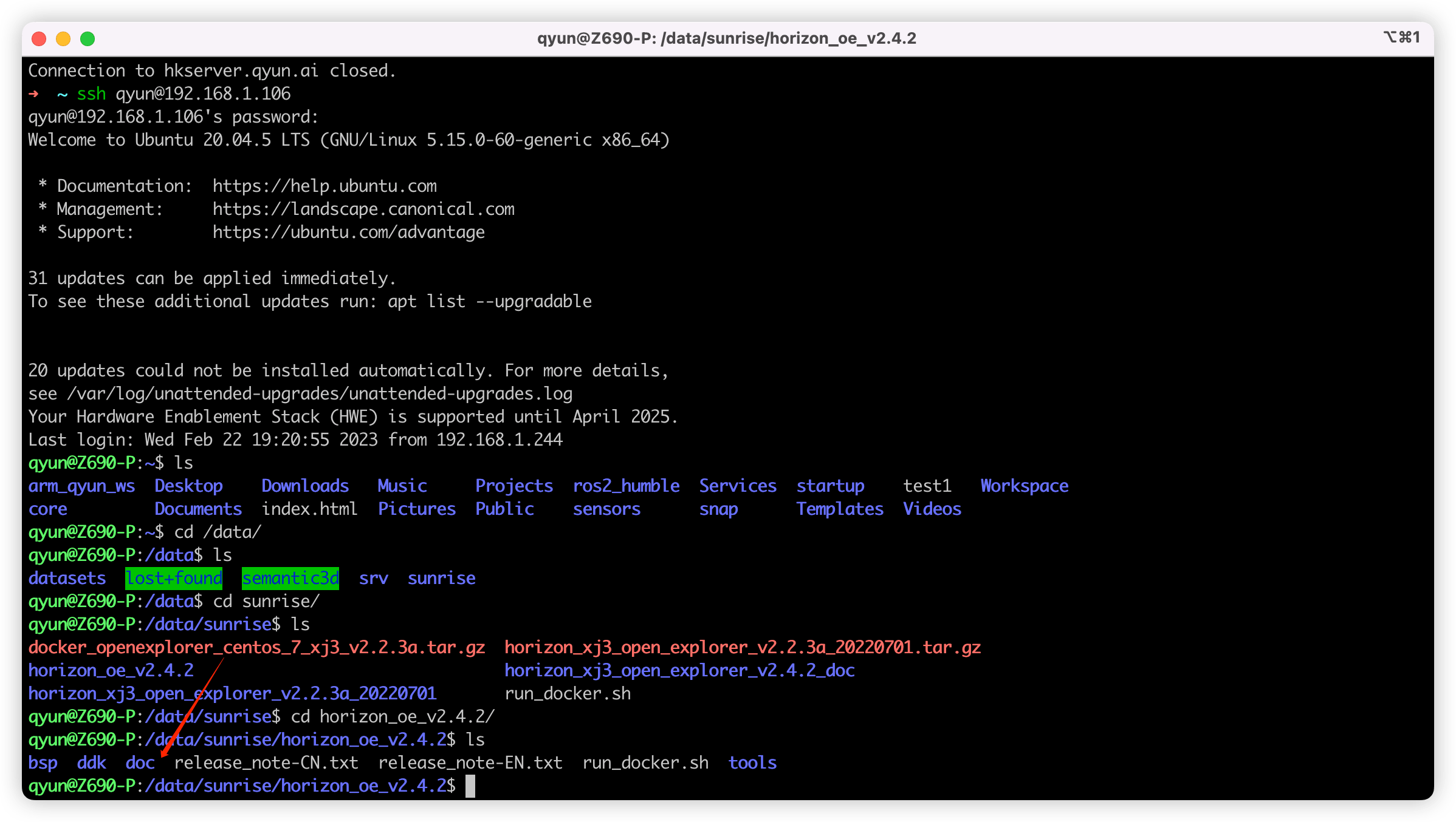
想要方便的查看离线文档可以通过 Python 来实现,在 doc 目录下执行:
python3 -m http.server 3000
这样就可以在本地的 0.0.0.0:3000 地址开启一个 http server,随后可以在本地浏览器使用 localhost:3000 或者其他电脑浏览器使用 {ip}:3000 来访问文档。
但是查看 文档 过后会发现,文档其实也没有那么的全面,讲的比较简单,尝试了一下中间坑还挺多的,社区里面关于这方面的帖子也不多12,因此想记录下我尝试的全流程,也可以作为对上面教程文档的补充。
下面主要分为三部分:
训练的环境配置。
如何基于官方的 COCO 数据集训练?这里就是指基于 mscoco 发布的包含 80 类的数据集。
如何基于自己的数据集进行训练?这里就是指自己建立的,自定义类别的,可能只有四五类,没有 80 类的数据集。
下方涉及到的一些代码、脚本和模型等,可以在 Github 仓库 中找到。
训练的环境配置
我自己环境配置如下:
OS: Ubuntu 20.04
Docker: 20.10.23
Nvidia Docker: 2.11.0-1
GPU: RTX3090
NVIDIA Driver Version: 515.65.01
CUDA Version: 11.7
OE Version: v2.4.2( gcc-9.3.0 For XJ3 )
因为我的开发是基于 Ubuntu 进行,训练是 GPU 进行的,所以这里只提及关于 Ubuntu + GPU 训练的环境配置,Windows 情况下,或者只有 CPU 的情况,我也没尝试过。
首先需要安装 Docker 以及 NVIDIA Docker,前者安装参考:Docker 安装文档,后者安装参考:NVIDIA Docker 安装文档。
参考官方 X3 芯片文档编写启动脚本 run_docker.sh 如下:
#!/bin/bash
export version=v2.4.2

export ai_toolchain_package_path=/data/sunrise/horizon_oe_v2.4.2

export dataset_path=/data/datasets

docker run -dt --runtime=nvidia -e NVIDIA_DRIVER_CAPABILITIES=compute,utility \
  -e NVIDIA_VISIBLE_DEVICES=all --shm-size="15g" \
   --restart=always --network=host \
    -v "$ai_toolchain_package_path":/open_explorer \
      -v "$dataset_path":/data \
        openexplorer/ai_toolchain_centos_7_xj3:"${version}"
其中参数解释如下:
version 代表 Docker 镜像版本,可选版本参考:资料下载专区
ai_toolchain_package_path 代表 OE 开发包的路径,指定 OE 包中 ai_toolchain 的路径也可以,但是我建议把整个 OE 包都挂进去得了,没啥差别。
dataset_path 代表训练需要的数据集路径,这里可以新建一个空的文件夹然后挂载进去,也可以把你所有的数据集都准备好,然后放到一个文件夹,然后挂进去,需要训练哪个后面指定哪个即可,我们这里方便起见可以选择前者(官方说如果这里指定为空可能会出问题,但是我测试发现挂载空文件夹不会有问题)。
docker run 部分就是启动一个 Docker 容器,其中比较重要的参数: -dt 可以让容器使用 Daemon 的方式启动一个交互式终端,可以保证容器一直存活不会 detach 后就被杀死,方便我们多次操作;--restart=always 可以在每次开机时自动重启容器,可以视自己的情况去掉或者改成 --restart=unless-stopped 等;--network=host 指定与宿主机器使用同一个网络,方便我们查看文档或者后面的网络结构。
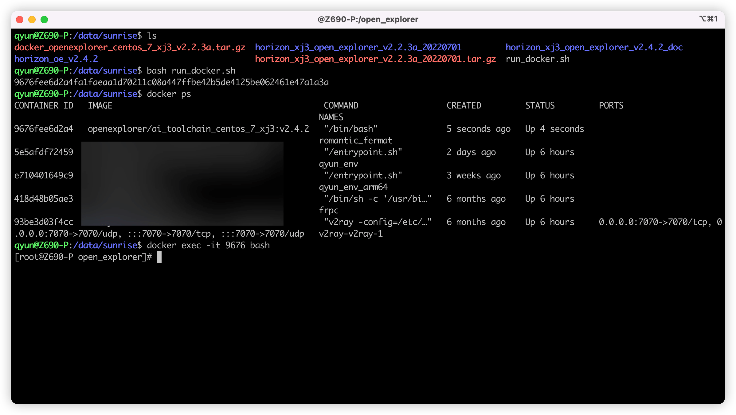
设置后即可打开终端,使用 bash run_docker.sh 启动容器,并使用 docker exec -it {container_id} bash 来连接容器进行操作,其中 container_id 可以通过 docker ps 或者上述脚本的返回值查看。
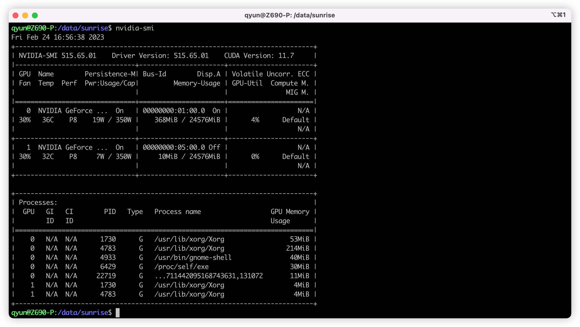
进入后可使用 nvidia-smi 验证一下,出现下方的信息即代表成功:
环境配置到此结束,终于可以开始训练和部署网络了。
训练 COCO 数据集并进行部署
数据准备
下方的操作均在上方启动的容器中进行,首先需要先 docker exec 进入容器中。
其中准备 COCO 数据集部分参考 官方文档部分,首先进入 /data 目录,然后新建一个文件夹 mscoco,下载数据集、解压即可。
# 进入之前挂载的 /data 目录
cd /data
# 创建一个目录来存储数据集
mkdir mscoco
# 下载 train2017.zip,即训练数据集
wget -c http://images.cocodataset.org/zips/train2017.zip
# 下载 val2017.zip,即验证数据集
wget -c http://images.cocodataset.org/zips/val2017.zip
# 下载 annotations_trainval2017.zip 即对应标签
wget -c http://images.cocodataset.org/annotations/annotations_trainval2017.zip
# 解压
unzip train2017.zip
unzip val2017.zip
unzip annotations_trainval2017.zip
随后进入 /open_explorer/horizon_model_train_samples 目录,如果这里你和我之前一样是挂载的整个 OE 包,那这个路径可能会长一些,例如我这里是 /open_explorer/ddk/samples/ai_toolchain/horizon_model_train_samples。
将数据集打包成 lmdb 格式,注意下方的 /data/mscoco 路径是我们之前存放数据集的路径:
# 转换训练集
python3 tools/datasets/mscoco_packer.py --src-data-dir /data/mscoco/ --target-data-dir /data/mscoco --split-name train --pack-type lmdb
# 转换验证集
python3 tools/datasets/mscoco_packer.py --src-data-dir /data/mscoco/ --target-data-dir /data/mscoco --split-name val --pack-type lmdb
运行完即打包成功,/data/mscoco 目录下会多出来 train_lmdb 和 val_lmdb 两个文件夹,即打包之后的训练数据集和验证数据集,也是网络最终读取的数据集。
修改配置文件
地平线提供的 HAT 工具链是一个类 mmdetion 的东西,模型定义、训练、验证都流程都定义在一个 config.py 文件中,官方提供的所有配置文件可以在 configs 目录下找到,FCOS 对应的就是 configs/detection/fcos 目录下的配置文件,方便起见,我们这里只考虑 fcos_efficientnetb0_mscoco.py ,关于配置的进一步讲解,可见官方文档:config 文件介绍。
在修改之前,最好先备份一下原件,可以作为对比,也方便回溯:
cp fcos_efficientnetb0_mscoco.py fcos_efficientnetb0_mscoco_back.py
要改的点有三个:
device_ids:这里代表的是你使用的 GPU 序号,如果只有一个 GPU 就只保留 [0],两个就是 [0, 1],以此类推。- 所有跟
./tmp_data有关的位置,这里相关的都是指定的数据集位置,官方举例是将数据集都放在了同 configs 同目录的tmp_data目录,但是我们放在了/data目录,因此要将所有的./tmp_data都改成/data float_trainer:这个参数是个 Dict,里面包含了一个num_epochs,代表我们训练多少轮,这里默认是 300,可以根据自己需求调整,例如 5、10、100 等。
开始训练!
训练很简单,一行命令即可:
# 进入 horizon_model_train_samples 目录
cd /open_explorer/ddk/samples/ai_toolchain/horizon_model_train_samples
# 开始训练
python3 tools/train.py --step float --config configs/detection/fcos/fcos_efficientnetb0_mscoco.py
如果不出意外,已经开始训练了,正常如下图所示:
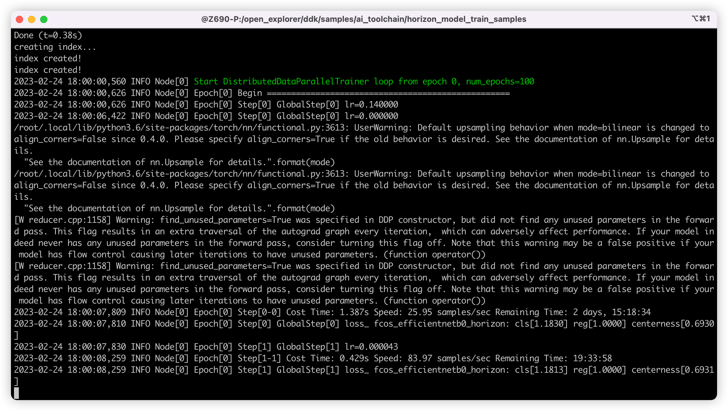
顺便说一下,这里推荐配合 tmux 工具来训练,可以让 session 在后台运行,防止意外中断,顺附一个 tmux 教程:Tmux 使用教程。
模型转换
训练的时间比较长,主要取决于数据集的大小,如果是 mscoco 这种大型数据集,一个 epoch 就要好久才行。
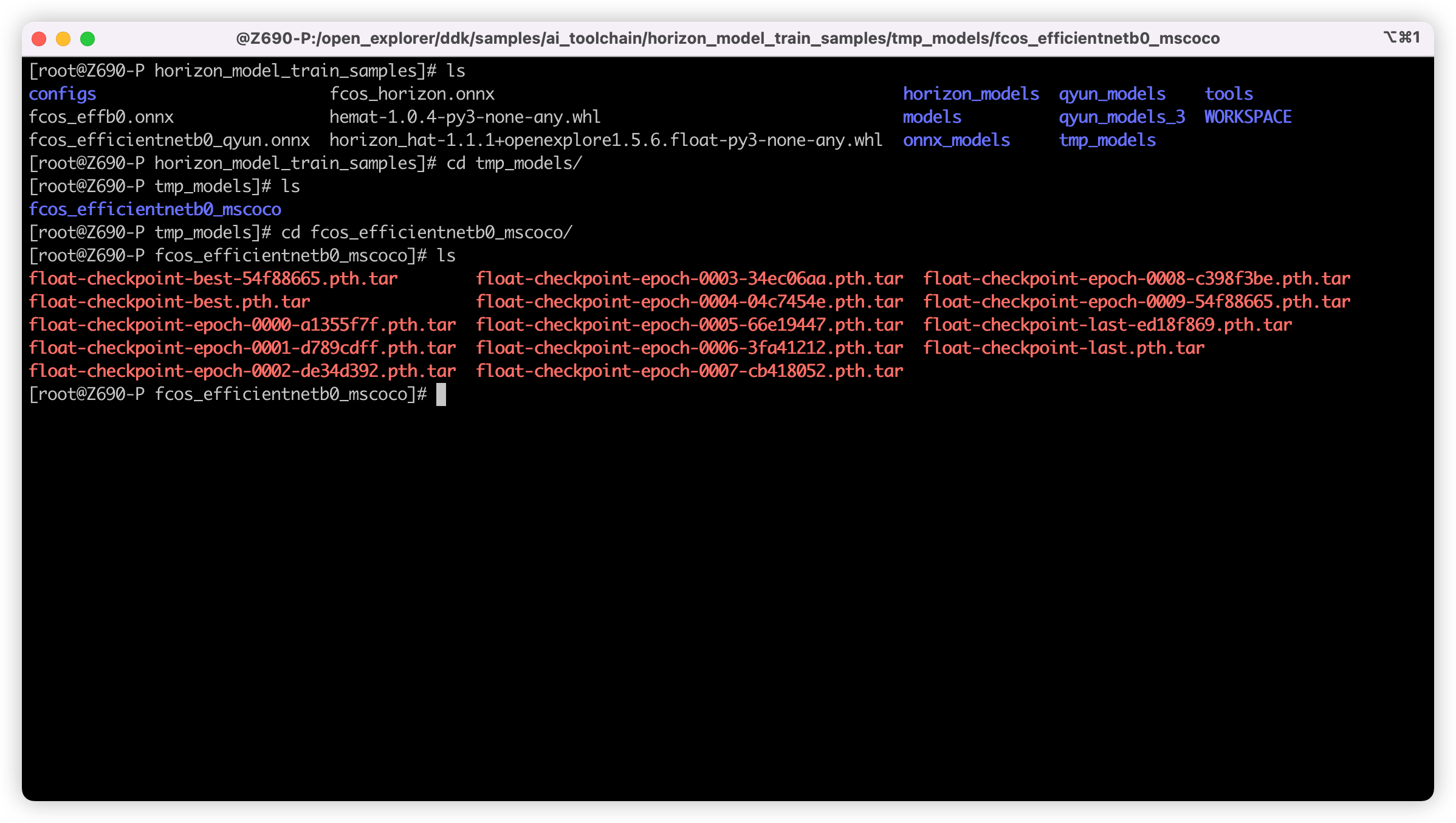
这里我训练了十轮就结束了,随后进入 tmp_models 目录,找到我们训练好的权重文件,如下图,这里的存放位置主要和配置文件中的 task_name 与 ckpt_dir 有关,可以按需修改:
接下来就是将权重文件导出成 ONNX 模型:
python3 tools/export_onnx.py --config configs/detection/fcos/fcos_efficientnetb0_mscoco.py --ckpt tmp_models/fcos_efficientnetb0_mscoco/float-checkpoint-best.pth.tar --onnx-name fcos.onnx
如上命令,将训练得到的 best 权重文件(float-checkpoint-best.pth.tar)导出成了 fcos.onnx 模型文件,这里也可以选择其他的权重,指定对模型路径即可。
接下来是使用地平线的工具链对 ONNX 模型进行量化,以便我们后面上板推理:
第一步,先移动一下得到的权重文件,方便后面的查找:
# 进入 horizon_model_train_samples 目录
cd /open_explorer/ddk/samples/ai_toolchain/horizon_model_train_samples
# 建立文件夹
mkdir -p ../horizon_model_convert_sample/08_customs
# 移动 onnx 模型过去
cp ./fcos.onnx ../horizon_model_convert_sample/08_customs
接下来就是那套标准的转换流程,可以参考官方教程:6.3 快速体验,还有大佬的指南:一文带你轻松走出模型部署新手村。
主要是涉及模型地址和数据集地址的时候需要改成我们对应的即可,其他的都默认就行,接下来给出我的几个脚本及精简后的转换配置文件:
- 01_check.sh
# 01_check.sh
set -e -v
cd $(dirname $0)

model_type="onnx"
onnx_model="../../../08_customs/fcos.onnx"
march="bernoulli2"

hb_mapper checker --model-type ${model_type} \
                  --model ${onnx_model} \
                  --march ${march}
- 02_preprocess.sh
# 02_preprocess.sh
set -e -v

cd $(dirname $0) || exit

python3 ../../../data_preprocess.py \
  --src_dir /data/mscoco/train2017 \
  --dst_dir ./calibration_data_yuv_f32 \
  --cal_img_num 50 \
  --pic_ext .yuv \
  --read_mode opencv \
  --saved_data_type float32
- fcos_efficientnetb0_config.yaml
# fcos_efficientnetb0_config.yaml
model_parameters:
  onnx_model: '../../../08_customs/fcos.onnx'
  march: "bernoulli2"
  layer_out_dump: False
  working_dir: 'fcos_test'
  output_model_file_prefix: 'fcos_test'
input_parameters:
  input_name: ""
  input_type_rt: 'nv12'
  input_type_train: 'yuv444'
  input_layout_train: 'NCHW'
  input_shape: ''
  norm_type: 'data_mean_and_scale'
  mean_value: 128.0
  scale_value: 0.0078125
calibration_parameters:
  cal_data_dir: './calibration_data_yuv_f32_qyun'
  cal_data_type: 'float32'
  calibration_type: 'max'
  max_percentile: 0.99996
compiler_parameters:
  compile_mode: 'latency'
  debug: False
  optimize_level: 'O3'
这里理论上只需要执行完 03_build.sh 脚本转换即结束,不出意外在同目录下会生成 fcos_test 目录,已经在其中可找到 fcos.bin ,这即是我们后续上板推理需要的模型文件。
模型推理
这里 Python 推理我参考了 X3M 板子上 /app/ai_inference/02_usb_camera_sample/usb_camera_fcos.py 目录下的推理脚本,直接上代码:
#!/usr/bin/env python3

import os
from hobot_dnn import pyeasy_dnn as dnn
from hobot_vio import libsrcampy as srcampy
import numpy as np
import cv2
import colorsys
from time import time

# detection model class names


def get_classes():
    return np.array(["person", "bicycle", "car",
                     "motorcycle", "airplane", "bus",
                     "train", "truck", "boat",
                     "traffic light", "fire hydrant", "stop sign",
                     "parking meter", "bench", "bird",
                     "cat", "dog", "horse",
                     "sheep", "cow", "elephant",
                     "bear", "zebra", "giraffe",
                     "backpack", "umbrella", "handbag",
                     "tie", "suitcase", "frisbee",
                     "skis", "snowboard", "sports ball",
                     "kite", "baseball bat", "baseball glove",
                     "skateboard", "surfboard", "tennis racket",
                     "bottle", "wine glass", "cup",
                     "fork", "knife", "spoon",
                     "bowl", "banana", "apple",
                     "sandwich", "orange", "broccoli",
                     "carrot", "hot dog", "pizza",
                     "donut", "cake", "chair",
                     "couch", "potted plant", "bed",
                     "dining table", "toilet", "tv",
                     "laptop", "mouse", "remote",
                     "keyboard", "cell phone", "microwave",
                     "oven", "toaster", "sink",
                     "refrigerator", "book", "clock",
                     "vase", "scissors", "teddy bear",
                     "hair drier", "toothbrush"])
    # return np.array(["tissue", "sock", "shoe", "cable", "bin"])

# bgr格式图片转换成 NV12格式


def bgr2nv12_opencv(image):
    height, width = image.shape[0], image.shape[1]
    area = height * width
    yuv420p = cv2.cvtColor(
        image, cv2.COLOR_BGR2YUV_I420).reshape((area * 3 // 2,))
    y = yuv420p[:area]
    uv_planar = yuv420p[area:].reshape((2, area // 4))
    uv_packed = uv_planar.transpose((1, 0)).reshape((area // 2,))

    nv12 = np.zeros_like(yuv420p)
    nv12[:height * width] = y
    nv12[height * width:] = uv_packed
    return nv12


def postprocess(model_output,
                model_hw_shape,
                origin_image=None,
                origin_img_shape=None,
                score_threshold=0.5,
                nms_threshold=0.6,
                dump_image=False):
    input_height = model_hw_shape[0]
    input_width = model_hw_shape[1]
    if origin_image is not None:
        origin_image_shape = origin_image.shape[0:2]
    else:
        origin_image_shape = origin_img_shape

    prediction_bbox = decode(outputs=model_output,
                             score_threshold=score_threshold,
                             origin_shape=origin_image_shape,
                             input_size=512)

    prediction_bbox = nms(prediction_bbox, iou_threshold=nms_threshold)

    prediction_bbox = np.array(prediction_bbox)
    topk = min(prediction_bbox.shape[0], 1000)

    if topk != 0:
        idx = np.argpartition(prediction_bbox[..., 4], -topk)[-topk:]
        prediction_bbox = prediction_bbox[idx]

    if dump_image and origin_image is not None:
        draw_bboxs(origin_image, prediction_bbox)
    return prediction_bbox


def draw_bboxs(image, bboxes, gt_classes_index=None, classes=get_classes()):
    """draw the bboxes in the original image
    """
    num_classes = len(classes)
    image_h, image_w, channel = image.shape
    hsv_tuples = [(1.0 * x / num_classes, 1., 1.) for x in range(num_classes)]
    colors = list(map(lambda x: colorsys.hsv_to_rgb(*x), hsv_tuples))
    colors = list(
        map(lambda x: (int(x[0] * 255), int(x[1] * 255), int(x[2] * 255)),
            colors))

    fontScale = 0.5
    bbox_thick = int(0.6 * (image_h + image_w) / 600)

    for i, bbox in enumerate(bboxes):
        coor = np.array(bbox[:4], dtype=np.int32)

        if gt_classes_index == None:
            class_index = int(bbox[5])
            score = bbox[4]
        else:
            class_index = gt_classes_index[i]
            score = 1

        bbox_color = colors[class_index]
        c1, c2 = (coor[0], coor[1]), (coor[2], coor[3])
        cv2.rectangle(image, c1, c2, bbox_color, bbox_thick)
        classes_name = classes[class_index]
        bbox_mess = '%s: %.2f' % (classes_name, score)
        t_size = cv2.getTextSize(bbox_mess,
                                 0,
                                 fontScale,
                                 thickness=bbox_thick // 2)[0]
        cv2.rectangle(image, c1, (c1[0] + t_size[0], c1[1] - t_size[1] - 3),
                      bbox_color, -1)
        cv2.putText(image,
                    bbox_mess, (c1[0], c1[1] - 2),
                    cv2.FONT_HERSHEY_SIMPLEX,
                    fontScale, (0, 0, 0),
                    bbox_thick // 2,
                    lineType=cv2.LINE_AA)
        print("{} is in the picture with confidence:{:.4f}".format(
            classes_name, score))
    #    cv2.imwrite("demo.jpg", image)
    return image


def decode(outputs, score_threshold, origin_shape, input_size=512):
    def _distance2bbox(points, distance):
        x1 = points[..., 0] - distance[..., 0]
        y1 = points[..., 1] - distance[..., 1]
        x2 = points[..., 0] + distance[..., 2]
        y2 = points[..., 1] + distance[..., 3]
        return np.stack([x1, y1, x2, y2], -1)

    def _scores(cls, ce):
        cls = 1 / (1 + np.exp(-cls))
        ce = 1 / (1 + np.exp(-ce))
        return np.sqrt(ce * cls)

    def _bbox(bbox, stride, origin_shape, input_size):
        # l t r b | h, w = t, r
        h, w = bbox.shape[1:3]
        yv, xv = np.meshgrid(np.arange(h), np.arange(w))
        xy = (np.stack((yv, xv), 2) + 0.5) * stride
        bbox = _distance2bbox(xy, bbox)
        # opencv read, shape[1] is w, shape[0] is h
        scale_w = origin_shape[1] / input_size
        scale_h = origin_shape[0] / input_size
        scale = max(origin_shape[0], origin_shape[1]) / input_size
        # origin img is pad resized
        # bbox = bbox * scale
        # origin img is resized
        bbox = bbox * [scale_w, scale_h, scale_w, scale_h]
        return bbox

    bboxes = list()
    strides = [8, 16, 32, 64, 128]

    # 各个 stride 找符合的模型
    for i in range(len(strides)):
        cls = outputs[i].buffer
        bbox = outputs[i + 5].buffer
        ce = outputs[i + 10].buffer
        scores = _scores(cls, ce)

        classes = np.argmax(scores, axis=-1)
        classes = np.reshape(classes, [-1, 1])
        max_score = np.max(scores, axis=-1)
        max_score = np.reshape(max_score, [-1, 1])
        bbox = _bbox(bbox, strides[i], origin_shape, input_size)
        bbox = np.reshape(bbox, [-1, 4])

        pred_bbox = np.concatenate([bbox, max_score, classes], axis=1)

        index = pred_bbox[..., 4] > score_threshold
        pred_bbox = pred_bbox[index]
        bboxes.append(pred_bbox)

    return np.concatenate(bboxes)


def nms(bboxes, iou_threshold, sigma=0.3, method='nms'):
    def bboxes_iou(boxes1, boxes2):
        boxes1 = np.array(boxes1)
        boxes2 = np.array(boxes2)
        boxes1_area = (boxes1[..., 2] - boxes1[..., 0]) * \
                      (boxes1[..., 3] - boxes1[..., 1])
        boxes2_area = (boxes2[..., 2] - boxes2[..., 0]) * \
                      (boxes2[..., 3] - boxes2[..., 1])
        left_up = np.maximum(boxes1[..., :2], boxes2[..., :2])
        right_down = np.minimum(boxes1[..., 2:], boxes2[..., 2:])
        inter_section = np.maximum(right_down - left_up, 0.0)
        inter_area = inter_section[..., 0] * inter_section[..., 1]
        union_area = boxes1_area + boxes2_area - inter_area
        ious = np.maximum(1.0 * inter_area / union_area,
                          np.finfo(np.float32).eps)

        return ious

    classes_in_img = list(set(bboxes[:, 5]))
    best_bboxes = []

    for cls in classes_in_img:
        cls_mask = (bboxes[:, 5] == cls)
        cls_bboxes = bboxes[cls_mask]

        while len(cls_bboxes) > 0:
            max_ind = np.argmax(cls_bboxes[:, 4])
            best_bbox = cls_bboxes[max_ind]
            best_bboxes.append(best_bbox)
            cls_bboxes = np.concatenate(
                [cls_bboxes[:max_ind], cls_bboxes[max_ind + 1:]])
            iou = bboxes_iou(best_bbox[np.newaxis, :4], cls_bboxes[:, :4])
            weight = np.ones((len(iou),), dtype=np.float32)

            assert method in ['nms', 'soft-nms']

            if method == 'nms':
                iou_mask = iou > iou_threshold
                weight[iou_mask] = 0.0
            if method == 'soft-nms':
                weight = np.exp(-(1.0 * iou ** 2 / sigma))

            cls_bboxes[:, 4] = cls_bboxes[:, 4] * weight
            score_mask = cls_bboxes[:, 4] > 0.
            cls_bboxes = cls_bboxes[score_mask]

    return best_bboxes


def print_properties(pro):
    print("tensor type:", pro.tensor_type)
    print("data type:", pro.dtype)
    print("layout:", pro.layout)
    print("shape:", pro.shape)


if __name__ == '__main__':
    models = dnn.load('./models/fcos.bin')
    # 打印输入 tensor 的属性
    print_properties(models[0].inputs[0].properties)
    # 打印输出 tensor 的属性
    print(len(models[0].outputs))
    for output in models[0].outputs:
        print_properties(output.properties)

    frame = cv2.imread("./kite.jpg")
    if frame is None:
        print("Image is not exist.")
    height, width = frame.shape[:2]
    print("height: ", height, "width: ", width)
    # 把图片缩放到模型的输入尺寸
    # 获取算法模型的输入tensor 的尺寸
    h, w = models[0].inputs[0].properties.shape[2], models[0].inputs[0].properties.shape[3]
    des_dim = (w, h)
    resized_data = cv2.resize(frame, des_dim, interpolation=cv2.INTER_AREA)
    nv12_data = bgr2nv12_opencv(resized_data)

    # Forward
    outputs = models[0].forward(nv12_data)
    # Do post process
    input_shape = (h, w)
    prediction_bbox = postprocess(
        outputs, input_shape, origin_img_shape=(height, width))

    if frame.shape[0] != height or frame.shape[1] != width:
        frame = cv2.resize(frame, (width, height),
                           interpolation=cv2.INTER_AREA)

    # Draw bboxs
    box_bgr = draw_bboxs(frame, prediction_bbox)

    cv2.imwrite("kite_with_bbox.jpg", box_bgr)
其实流程还是蛮简单的,就是 加载模型 -> 读取照片 -> Resize 照片到模型推理尺寸 -> 转化为 NV12 输入格式 -> 拿到输出 outputs -> 对数据集进行后处理得到 bbox 与 classes 等数据 -> Resize 照片到原尺寸绘制框 -> 写照片。
大家拿脚本推理的时候,只需要改变 models 和读取照片的位置即可,这里我采用的示例图片是在模型转化后测试推理使用的,可以在 OE 包的如下路径找到 ai_toolchain/horizon_model_convert_sample/01_common/test_data/det_images/kite.jpg。
接下来就是运行脚本进行推理,得到的推理结果如下:
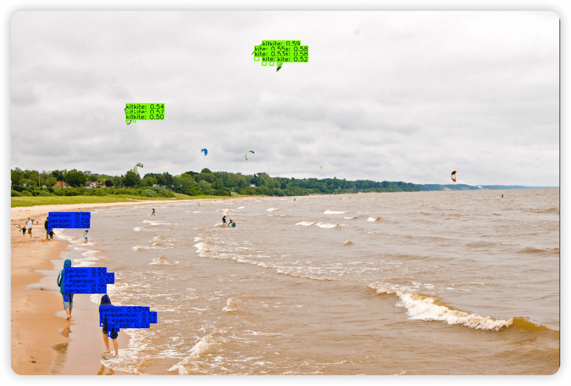
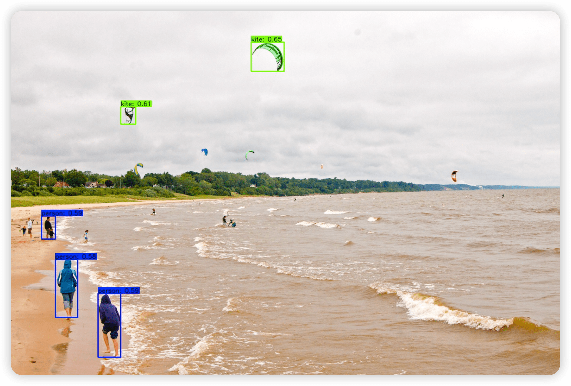
为什么结果是这样的,起初我认为是我推理脚本写错了,因此我直接将权重替换为官方的权重,得到的结果如下:
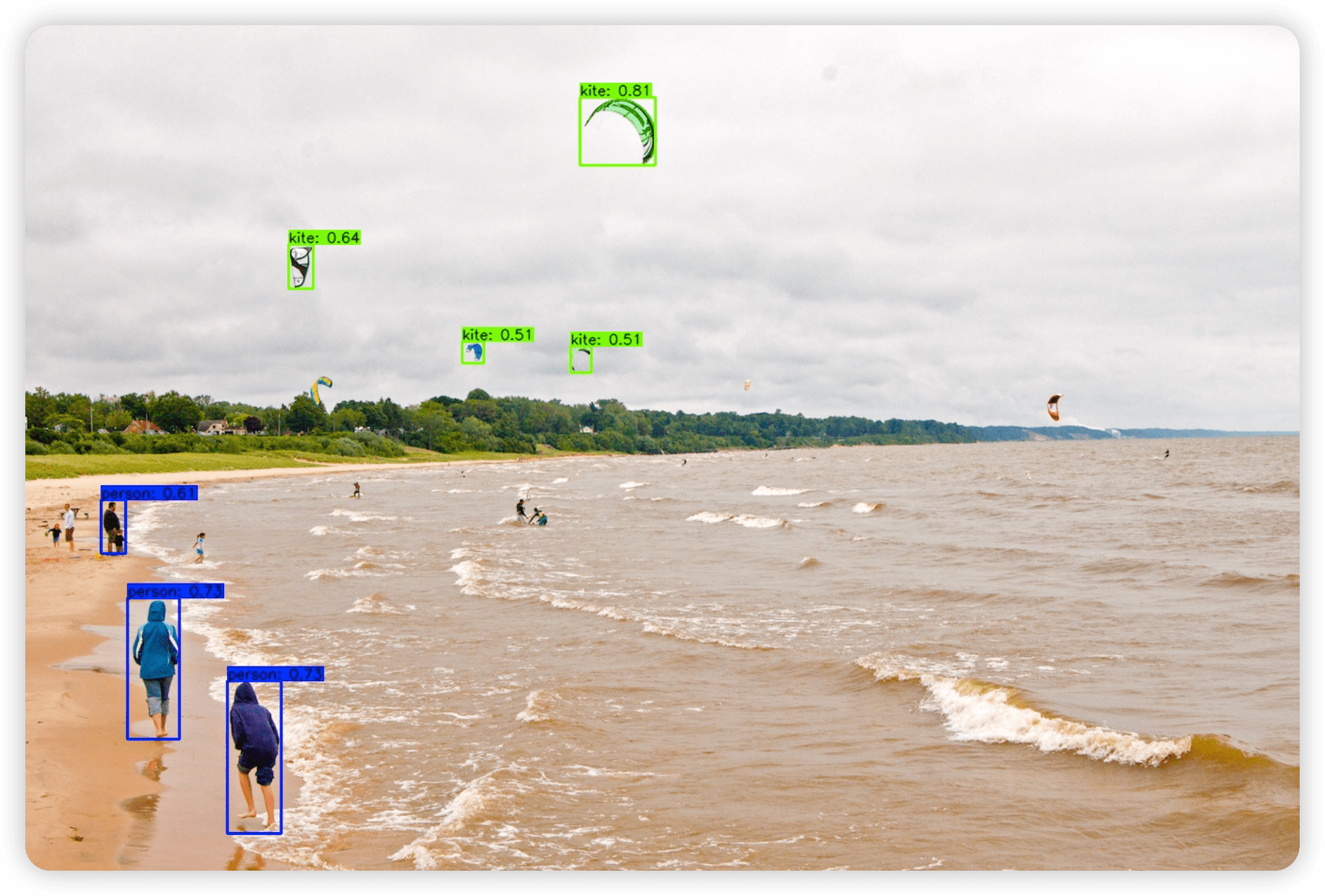
很显然,这次的推理是正确的,也就是说明,脚本是没问题,只是权重出了问题,因此我又仔细检查了训练和模型转换的各个步骤,但都没有发现问题。同时,使用官方提供的 mapper 目录下原 onnx 进行转换后,也是没有问题的。那么问题在哪里呢?
查找问题
因为通过上面的排除可以确定,转化这个过程是没什么问题的,那也就只能是模型定义和训练中出现的问题,但是上面的效果又明显不是训练过拟合或者欠拟合导致的,因为框的位置是大致对的,就是太多了,而且太小了,因此我怀疑是模型上出了问题,可能是有节点不一致。
确定了方向,接下来我首先对官方原 onnx 模型文件和我自己训练得到的 onnx 模型使用了 01_checker.sh 脚本来进行检查,因为他会输出模型中的各个层,对比结果如下:
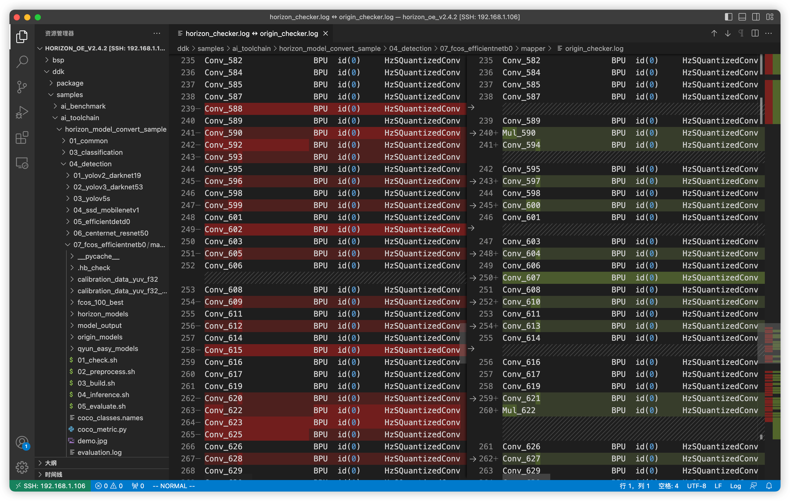
左侧是我自己训练得到的模型,右侧是我官方提供的模型,可以发现,两者存在差异,其实就是官方模型相比于训练得到的模型会多了几个 Mul 节点。
接下来进一步使用 netron 工具对两个模型进行对比,有区别的对比结果如下图所示:
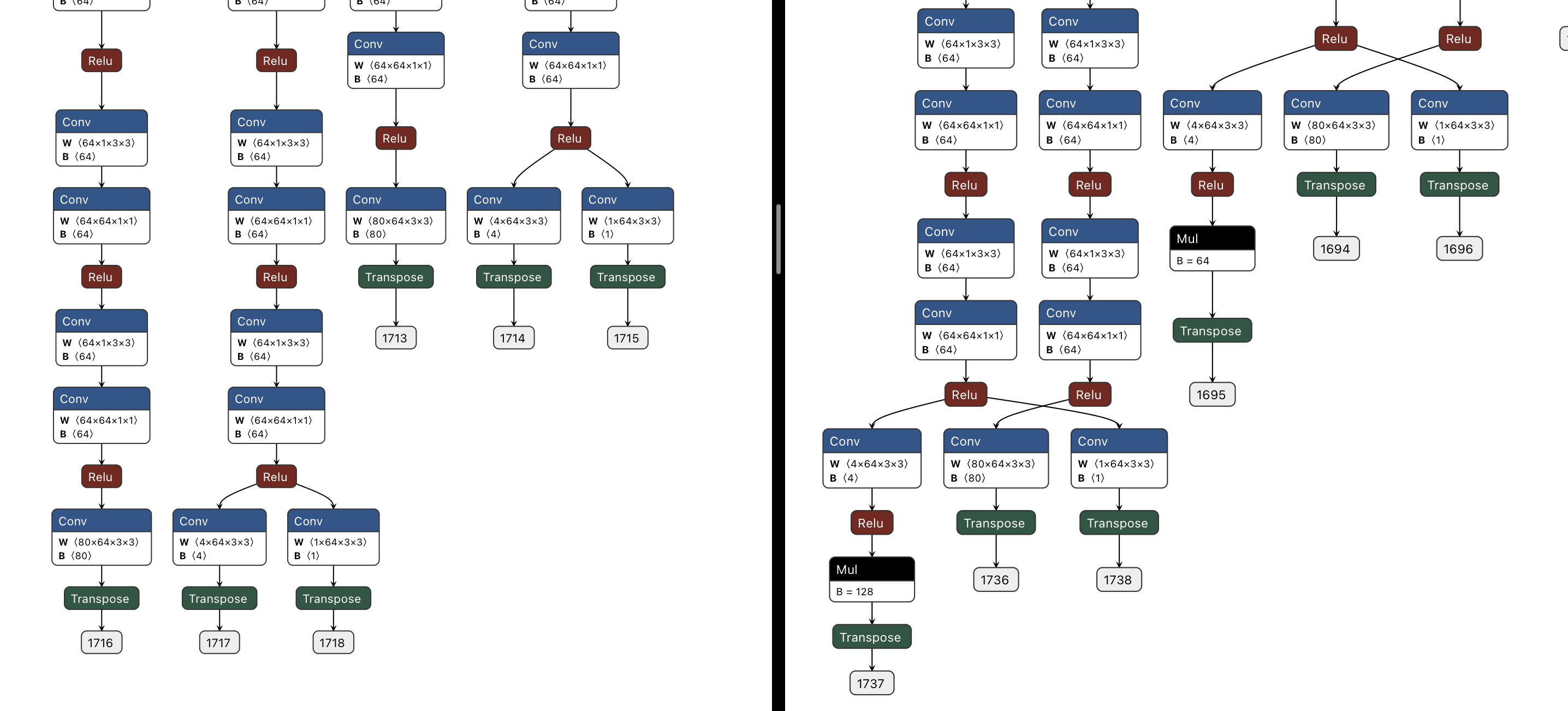
左侧为自己训练的模型,右侧为官方模型。可以看到只有 bbox 信息(对于 FCOS 为(l, t, r, b)四元组)在输出时两个模型有区别,多了一步 Relu 激活函数和 Mul 节点,其他的经过对比没有区别。
同时观察发现,这里 Mul 节点对应的数值,其实是对应的 stride(这个大家可以使用 netron 去看看)
知道了问题所在,解决方案就有了,只需要改动下面这一行即可:
# Decode 函数中获取数据的部分
# 各个 stride 找符合的模型
    for i in range(len(strides)):
        cls = outputs[i].buffer
        bbox = outputs[i + 5].buffer * strides[i]  # modified
        ce = outputs[i + 10].buffer
        scores = _scores(cls, ce)
很好理解,对 bbox 获得的原始数据乘了 strides[i],这里我没有处理 Relu 函数,因为即使是负数,OpenCV 绘制也是不会出问题的。
再次运行获得的推理图如下,这次正常了:
至此,训练 mscoco 数据集模型并进行部署就算结束了,接下来我们看看如何来处理自己得到的数据集。
训练自采集数据集
对于自采集数据集,最可能是数据处理打包、以及配置文件的配置这两部分存在问题,剩下的模型检查、校准数据准备、模型转化、以及上板推理部分可以说是根本没区别,所以就着重讲一下数据准备和配置部分。
数据准备
首先数据准备要准备 COCO JSON 格式,他是跟通用 JSON 格式也是有区别的,这个就不详述了。
然后方便起见,可以复用官方的 mscoco_packer.py 脚本,我们把数据集也存为 train2017、val2017 和 annotations 三个文件夹,例如存在放在 /data/selfcoco 目录下,类似于下面:
[root@Z690-P selfcoco]# tree
.
├── annotations
│   ├── instances_train2017.json  # 训练集的 label
│   └── instances_val2017.json    # 验证集的 label
├── train2017   # 训练集照片
└── val2017     # 验证集照片
这时候如果我们按照之前的操作,直接使用 mscoco_packer.py 脚本进行打包,会报错如下:
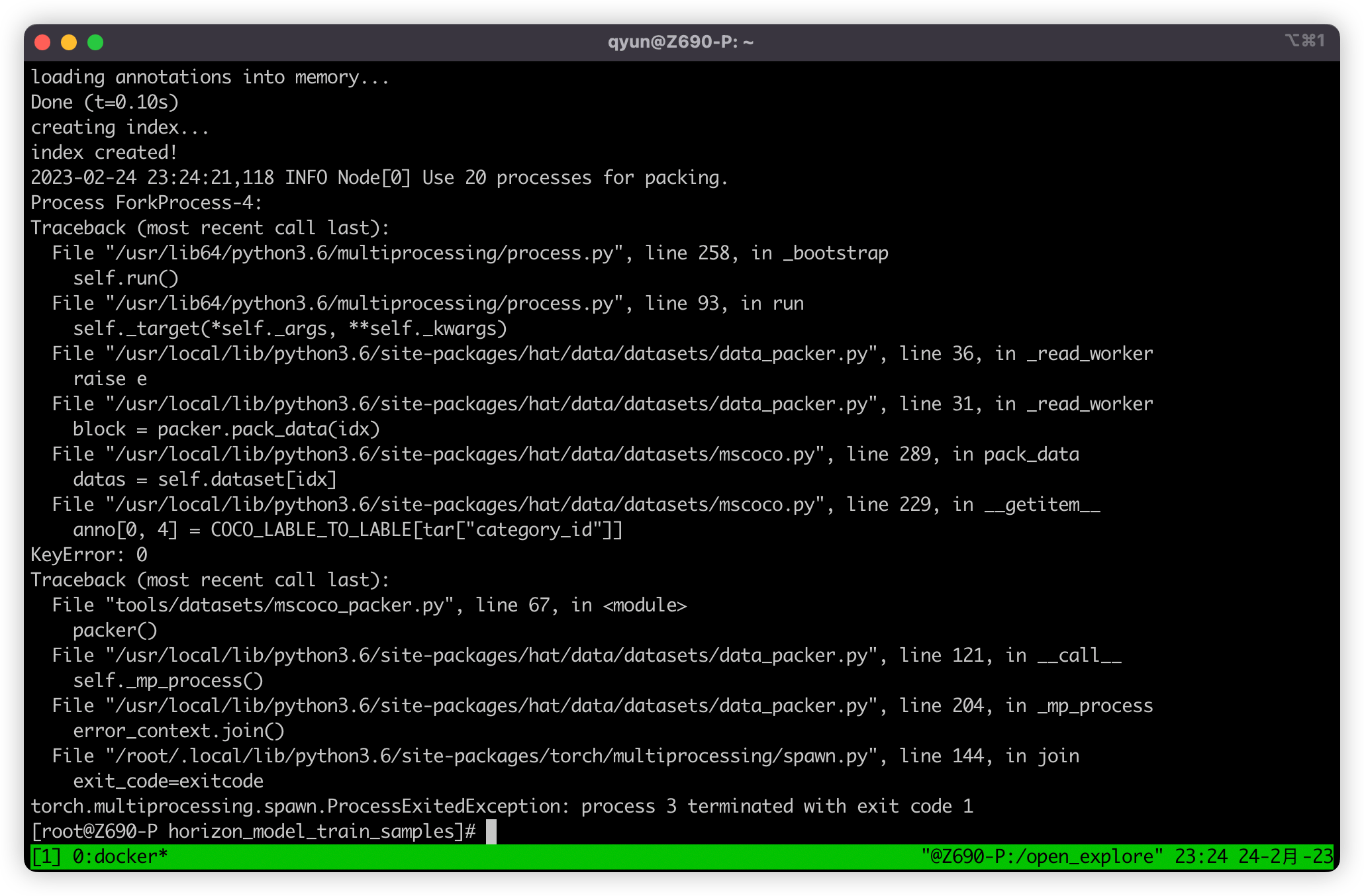
报错大意就是访问了字典一个不存在的键,直接查看报错的位置,位于 /usr/local/lib/python3.6/site-packages/hat/data/datasets/mscoco.py,查看后发现 COCO_LABLE_TO_LABLE 这个字典是一个类别的映射,因为 mscoco 数据集类别包含 80 类,按顺序来是 [0, 80),但是 mscoco 数据集原数据集类别序号范围为 [1, 90],但是其中只有 80 个类别序号,所以需要做一个 [1, 90] -> [0, 80) 的类别映射,但是如果我们自制的数据集没有这个类别映射的需求,就不需要映射,把涉及到这个 Dict 的两行都去掉即可。
Btw:🤣 这里的 COCO_LABLE_TO_LABLE 是不是拼错了,要拼 LABEL 的?
# 229 行
# anno[0, 4] = COCO_LABLE_TO_LABLE[tar["category_id"]]
anno[0, 4] = tar["category_id"]
# 327 行
# np.array([[COCO_LABLE_TO_LABLE[tar["category_id"]]]])
np.array([[tar["category_id"]]])
随后打包即可
# 转换训练集
python3 tools/datasets/mscoco_packer.py --src-data-dir /data/selfcoco --target-data-dir /data/selfcoco --split-name train --pack-type lmdb
# 转换验证集
python3 tools/datasets/mscoco_packer.py --src-data-dir /data/selfcoco --target-data-dir /data/selfcoco --split-name val --pack-type lmdb
配置文件修改
配置文件除了之前提到的三处需要修改,配置文件中还需要修改与类别相关的参数,大概有如下几个:
num_classes:这里就是一个全局变量类别数,例如我这里有五类 [0, 5),那改为 5 即可。model:model 参数中还有很多涉及到 80 的,经过我查看源码后,发现这些 80 的位置都应该改成 num_classes 参数才可以,例如 model 中的 loss_cls 参数,其中的 num_classes 参数值 80+1 就需要改为num_classes + 1,post_process 参数中的 num_classes 参数值 80 也应该改为num_classes,这里我认为是官方的疏忽,应该是忘记改了。
修改完后就可以按之前的方法进行训练了:
# 进入 horizon_model_train_samples 目录
cd /open_explorer/ddk/samples/ai_toolchain/horizon_model_train_samples
# 开始训练
python3 tools/train.py --step float --config configs/detection/fcos/fcos_efficientnetb0_mscoco.py
校准数据准备
这里预处理的数据也应该选择我们训练的数据子集,需要修改一下,剩下的都不需要变:
# 02_preprocess.sh
set -e -v

cd $(dirname $0) || exit

python3 ../../../data_preprocess.py \
  --src_dir /data/selfcoco/train2017 \ # 重要
  --dst_dir ./calibration_data_yuv_f32 \
  --cal_img_num 50 \
  --pic_ext .yuv \
  --read_mode opencv \
  --saved_data_type float32
推理代码修改
这里需要修改 get_classes 函数返回的类别名,改成自己对应的类别 List.
推理得到结果如下:
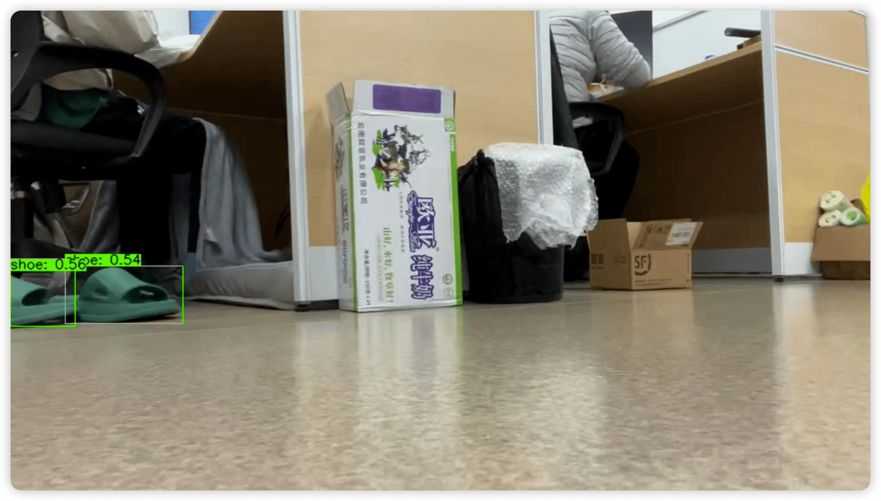
可以看到,识别可以正常的工作(因为我选的训练数据集有点捞,所以过拟合比较严重,就选了一张凑合能看的图,大家见谅)。
后言
这样我们就完成了 FCOS 网络的训练和部署,但是基于 Python 的推理可能有点慢,大家可以参考 ai_benchmark 等部分进行 C++ 推理,主要关键就是 PostProcess 后处理部分,不过之前 开发者直播KE——AI板端部署实践 张老师已经讲过一部分 API,如果大家有兴趣,我后面也可以给大家出个帖子讲讲 🤗。
探索的这几天,给我的感觉是,地平线做了很多,写了很多有用的工具、包,但是文档还是不够完善,而且文档有些混乱,版本比较混乱,位置比较混乱、等等,容易找不到、无从下手等等。
例如对于 FCOS 这部分的文档就很欠缺,对于 FCOS 训练配置的各个选项的详解,大家看到时候可能会有很多问题,例如:
- 如何使用 CPU 进行训练而不是 GPU?
- 如何基于已有的模型进行迁移训练?中断训练后可以再继续进行吗?
- 可以 freeze 一部分参数进行 fine-tuning 吗?
- 训练时有数据增强吗?如果不需要可以去掉吗?
不过现在也是在慢慢完善,不断进步,希望可以把这些好用的东西都能让大家快点方便的用起来。
文中涉及到的一些代码、脚本和模型等,可以在 Github 仓库 中找到。
文章同步发布在我的博客:https://blog.zzsqwq.cn